Implicit, deformable thin-sheet dynamics simulation engine

Abstract

This project explores the simulation of the dynamics of thin-sheets, focusing on achieving realistic folding and bending behaviors particularly on stiff materials like paper. Building upon the CS 184 Project 4 cloth simulation framework, we implemented a robust physics engine that addresses key stability challenges in material simulation. We replaced the rectangular grid structure with support for arbitrary triangle meshes loaded from OBJ files, and introduced constraint-based energy functions. To overcome stability issues with explicit Verlet integration, we implemented a semi-implicit Euler solver with TinyAD for automatic differentiation, enabling efficient computation of derivatives and Hessians for our constraint system. We enhanced realism through angle-based bending constraints and plastic deformation modeling. While we initially planned to implement full origami-like paper simulations, in the interest of time we narrowed our scope to focus on the underlying physics of paper-like materials and ended up being able to simualte general thin sheets. Our approach successfully demonstrates that cloth simulation techniques can be adapted to model stiffer materials with realistic folding behavior without implementing complex remeshing or explicit fold creation.

Technical Approach

Our project originally set out to simulate origami through the realistic thin-sheet engine in "Folding and Crumpling of Adaptive Sheets" by Pfaff et. al.. However, its nonlinear solver and remeshing algorithm proved too difficult to implement in four weeks, so we instead focused on the methods outlined in two simpler papers: "Large Steps in Cloth Simulation" by Baraff and Witkin, and "Discrete Shells" by Grinspun et al. On top of the CS184 Project 4 (cloth simluation) GUI, this included: support for arbitrary triangle meshes, more advanced force and constraint models, and the improved numerical stability of a semi-implicit integrator.

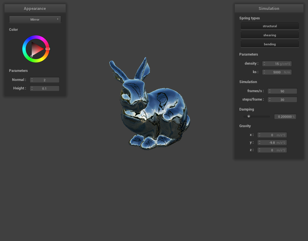
1. Triangle Mesh Support

We began by replacing Project 4's grid-based cloth structure with a general mesh system capable of loading arbitrary triangular meshes from .obj files. We used the TinyOBJ library to parse these input files and into lists of spatial positions, UV coordinates, and faces.

Note that if UV coordinates are not provided in the .obj file, we make it so each vertex has different UV coordinates for each triangle it is a part of. For a triangle described by vertices \(A,B,C\) (in CCW order), \(A\)'s UV coordinates are \((0,0)\), \(B\)'s UV coordinates are \((\|B-A\|,0)\), and \(C\)'s UV coordinates are \(\left(\text{proj}_{B-A}(C-A),\text{dist}(C, B-A)\right)\).

2. Constraint Formulation

In constrast to Project 4's spring-network approach, we found in the literature most approaches to cloth simulation define simulation-wide energy terms that stem from violations of physical constraints (or are directly formulated from theory). This is the approach taken in Baraff and Witkin: for each physical property we wish the system to obey, we formulate a constraint function \(\mathbf{C(\vec{x})}\) that outputs either a vector or scalar quantity that represents the violation of the constraint in configuration \(\vec{x}\) (all of the particles positions). We then define a scalar energy associated with this constraint and an associated tunable parameter \(k\):

\[ E_C = \frac{k}{2} \mathbf{C(\vec{x})}^\top \mathbf{C(\vec{x})} \]

The cloth naturally proceeds toward the minimum energy configuration, each particle \(\mathbf{x}_i\) guided by a force (as described in Baraff and Witkin):

\[ \mathbf{f}_i = -\frac{\partial E_C}{\partial \mathbf{x}_i} = -\frac{k}{2} \frac{\partial \mathbf{C(\vec{x})}}{\partial \mathbf{x}_i} \mathbf{C(\vec{x})} \]

More concretely, the stretching constraint is formulated per-triangle as an approximate metric of the deviation of a triangle \((\mathbf{x}_1, \mathbf{x}_2, \mathbf{x}_3)\)'s area \(a\) from the rest area (calculated using UV coordinates):

\[\begin{pmatrix} \mathbf{w}_u \quad \mathbf{w}_v \end{pmatrix} = (\mathbf{x}_2 - \mathbf{x}_1 \quad \mathbf{x}_3 - \mathbf{x}_1) \begin{pmatrix} u_2 - u_1 & u_3 - u_1 \\ v_2 - v_1 & v_3 - v_1 \end{pmatrix}^{-1} \] \[ \mathbf{C(\vec{x})}_{\text{stretch}} = a \begin{pmatrix}||\mathbf{w}_u|| - 1 \\ ||\mathbf{w}_v|| - 1\end{pmatrix} \] (intution: scaling of normalized basis functions \(\mathbf{w}_u, \mathbf{w}_v\) must cause stretching)

Unsurprisingly, shearing is quite similar and is also formulated per-triangle in terms of the same basis vectors:

\[ \mathbf{C(\vec{x})}_{\text{shear}} = a \mathbf{w}_u(\mathbf{\vec{x}})^\top \mathbf{w}_v(\mathbf{\vec{x}}) \] (intution: non-orthogonality of normalized basis functions \(\mathbf{w}_u, \mathbf{w}_v\) must cause shearing)

Bending is instead formulated per-pairs of triangles in terms of the current and rest angles \(\theta, \bar{\theta}\) between their normals (\(e\) is the length of the triangle edge and \(h(e)\) is the 1/3 the average areas of the two triangles):

\[ \mathbf{C(\vec{x})}_{\text{bend}} = \frac{\|e\|}{\|h_e\|}(\theta - \bar{\theta}) \] (intution: deviation from rest angle)

We found that the formulation of \(\theta\) in terms of either cosine or tangent \(\mathbf{x}_i\) greatly affected numerical stability.

Combined, these constraints give rise to forces that can be time-integrated to simulate physical dynamics.

3. From Explicit to Implicit Integrators

For non-stiff systems such as floppy cloth, the constraints combined with the original Verlet integrator work quite well:

However, when increasing the constraint coefficients to make the cloth highly-stretch/shear resistant like plastics, papers, or metals, the integrator would fail to converge without an incredibly small timestep. This made simulating any reasonable-length sequence impractical. Again drawing from Baraff and Witkin, we replaced the Verlet integrator with a semi-implicit Euler integrator that has much, much better stability properties, allowing us to integrate highly stiff systems with large timesteps.

Semi-implicit Euler is a linearized variant of the more advanced Backward Euler (BE), with the benefit of being symplectic: it approximately conserves the energy of the system, which is highly desirable in physical simulation. Our update equation can be seen as the standard semi-implicit Euler equation mentioned in Baraff and Witkin with the additional simplification that forces do not depend on velocity: \(\frac{\partial f}{\partial v} = 0\). (In reality forces like damping do, but we omit this term for simplicity without much impact):

\[ \left(\mathbf{I} - \frac{h^2}{m} \frac{\partial \mathbf{f}}{\partial \mathbf{x}}\right) \Delta \mathbf{v} = \frac{h}{m} \left(\mathbf{f}_0 + h\frac{\partial \mathbf{f}}{\partial \mathbf{x}} \mathbf{v}_0\right) \]

Where \(h\) is the timestep and \(m\) is the particle mass. Notice that there is no explicit formula for \(\Delta \mathbf{v}\): we must solve this \(\mathbf{A}\vec{x} = \vec{b}\) system at each timestep to find the velocity update then use that to update this positions. We do this using either an LDLT or Conjugate Gradient solver, which both exploit the sparsity pattern of this problem: the force on \(\mathbf{x}_i\) nearly only depends on \(\mathbf{x}_i\).

Implementing this required some structural changes to our codebase:

• Switch from updating positions to updating velocities, then positions with a linear approximation
• Switch from CGL to Eigen, to be compatible with most solvers
• Switch from computing derivatives by hand to using TinyAD

The first two were not much effort, but the third was one of our biggest challenges: observe in the implicit update function the presence of force derivatives. We know the forces depend on the derivatives of constraint functions, so we actually need the Hessians of them. These are far too difficult to compute by hand, so we rewrote all of the energy functions in TinyAD's autodiff paradigm, which then computed gradients, Jacobians, and Hessians automatically. We could then use these in a solver to compute the velocity update. While this added some computational overhead, it at least guarantees correctness of the expressions and saves us a lot of effort.

Though it might look wonky without damping, we were able to achieve the paper-like behavior where it "stands" on one bent edge instead of completely draping over the sphere.

4. Damping

Damping gets a pretty thorough treatment in Baraff and Witkin: each constraint force has an associated damping force that has velocity dependence, so the Euler step gains two additional terms to account for this in the presence of \(\Delta v\). However, we did not have time to work through this, and instead found a simple velocity-dependent scale factor (exactly like what is used in Project 4) works quite well:

5. Plastic Deformation

To model permanent modifications to material structure induced by forces, we introduced a simple model of plastic deformation. In real materials, repeated folding or excessive bending can cause permanent folds, creases, and tears, and it no longer returns to its original state. So, we allow the rest dihedral angle \(\bar{\theta}\) between adjacent triangles to update when the bending exceeds a certain threshold.

Specifically, during each simulation step, if the absolute difference between the current dihedral angle and the rest angle exceeds a plasticity threshold (\(\delta_\text{plastic}\)), we update the rest angle to partially "follow" the current angle:

\[ \bar{\theta} \leftarrow (1 - \alpha)\bar{\theta} + \alpha\theta \]

6. Animation

To show materials interacting with moving objects (such as being folded or crushed), we took the static objects from Project 4 and added animation parameters: each object now has a set of spline points that trace the path it follows over time. Additional parameters like the radius of a sphere or the normal of a plane are also animated. This caused some issues with collisions: if a point collides with it, the correction vector now needs to include the distance the object will be updated due to animations. Even then, large forces can cause materials to pass through collision objects, which can currently only be avoided with small-enough timesteps.

Here we have two animated planes crushing a pre-folded piece of paper/plastic, but there are still issues with clipping in collisions:

Results

Problems Encountered

• Instability of Explicit Integrators

  As discussed, the Verlet integrator was far too unstable to be used on stiff systems so we replaced it with semi-implicit Euler.

• Implicit Integrator Performance Issues

  The linear solve at each timestep adds considerable overhead and forced us to reduce the size of our meshes, so we used faster Conjugate Gradient or LDLT-based methods. Even the, it is still tens of times slower than an explicit method.

• Complex Collision handling

  The crumpled meshes have difficult geometry for collisions when moving, so we reduced the timestep to make it more accurate. If we had more time, we would like to implement more advanced collision schemes such as BVH.

• Scaling issues with floating point We initially had the meshes be 1mx1m to start; this resulted in edge lengths near 0.005 meters, which cause issued with derivatives. 1e-3 squared is 1e-6, which is not so far from machine epsilon. Combined with floating point errors in multiply and divide, the gradients become quite noisy and unstable. To fix this, we normalized the edge lengths and masses to be 1, and scaled everything up accordingly. This allowed us to achieve our best timestep of around 1.5ms.

Lessons Learned

• Numerics is hard

  Seemingly small changes in coefficients caused wildly different stability properties in the integrator, which was difficult to debug when the systems were large. And on small systems we couldn't even reproduce the problem! We wish there was an easier way to debug systems like this; we tried various C++ debuggers but they often made the program unusably slow. We also didn't dive into the math behind Conjugate Gradient and LDLT decomposition-based methods, so this is kind of a black box for us.

• Knowing when to give up

  We spent a long time trying to derive the Hessians of constraint functions analytically, but eventually gave up and used autodiff. Looking back, we should have done this sooner because matrix calculus is very complicated sometimes. Although, we were also afraid that autodiff would add too much overhead, but it ended up being ok.

• Simple is better than nothing

  We spent time trying to get "proper" force-based damping functions to work, but they made the integrator explode. When we tried the simple velocity-damping, it worked quite well--maybe even well enough that we wouldn't have spent time on the more advanced version. So we should have started with the basic verison, and then added to it if we thought it was necessary.

Resources

• (Paper) Discrete Shells: https://www.cs.columbia.edu/cg/pdfs/10_ds.pdf
• (Paper) Large Steps in Cloth Simulation: cs.cmu.edu/~baraff/papers/sig98.pdf
• (Library) CGL Vectors Library: cs184.eecs.berkeley.edu/sp25/resources/cgl-vector-docs/
• (Library) TinyAD Library: github.com/patr-schm/TinyAD
• (Code) CS 184 Project 4 Starter Code

Team Contributions